If you're going to be working in finance, without a doubt you will be analyzing numbers over a period of time. This can be to look at how a business performed historically or to financially model out future projections. Oftentimes, this analysis is built at a very detailed level (by days or months) and then summarized (by quarters or years). As a result, a foundational skill everyone should learn to do quickly is how to lay out time series and quickly summarize it.
There are a couple of ways to do this and everyone will have their preference. I will give you my preference at the end (which I believe is a little harder to learn, but more powerful in the long run).
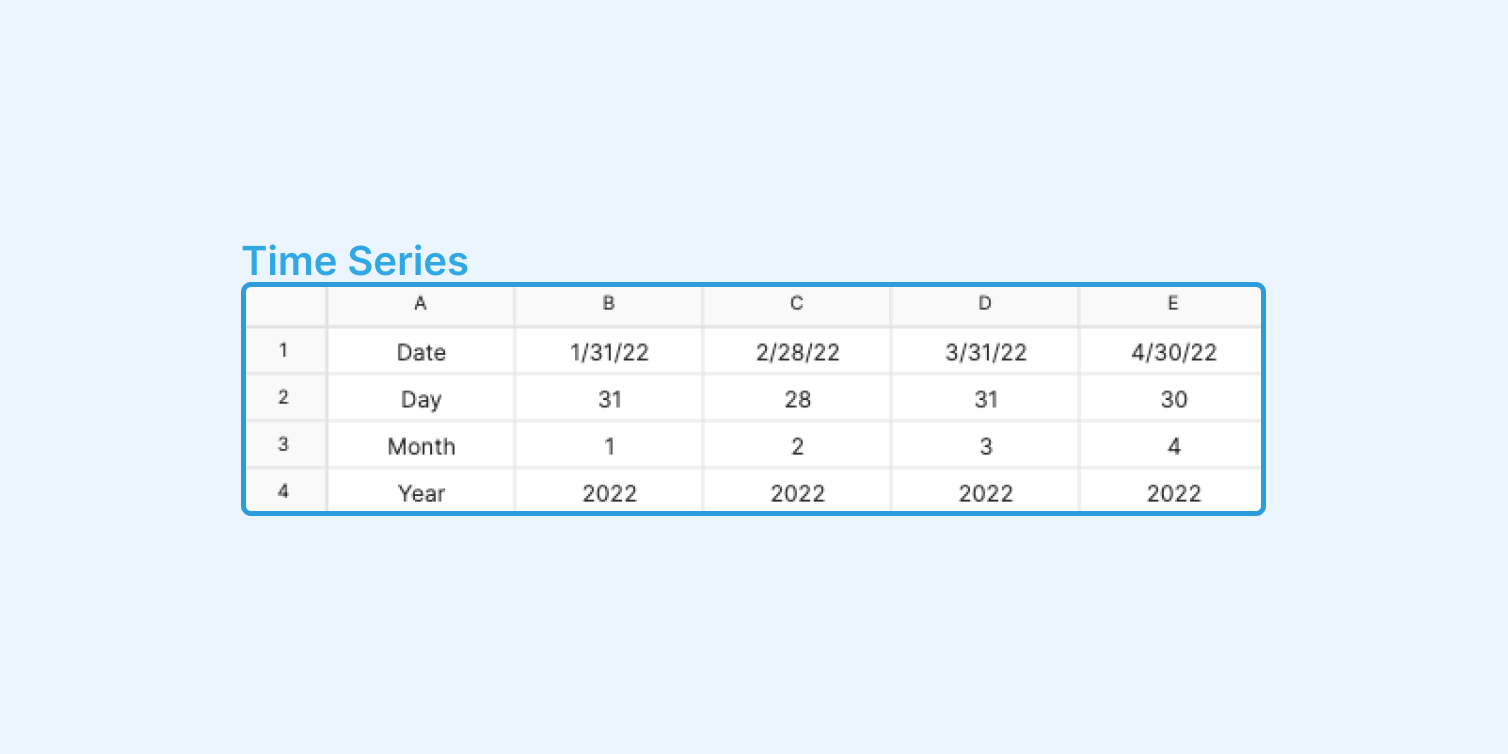
One formula that comes in very handy in time series that’s universal is =EOMONTH(Start_date, Months). There are more precise date formulas like EDATE or Date, however, in my experience, most of the time you are working with months at the most granular detail. EOMONTH standardizes how all the months are treated, and in this case, it returns the last day of every single month. Furthermore, once you have a start date, you can create a time series by month very easily by adding one month to the prior month. Below is how I set up time series if I end up summarizing the data using SUMIFS (you don't need rows 1-3 depending on what formula you use).
**First method: Pivot Tables**
If your data has a corresponding date, you can create a pivot table. The downside to this is that it's harder to format your summary sheet and it’s harder to trace back and audit the file. You have to trust that there are no mistakes (while Excel doesn't make mistakes, there's plenty of room for human error!).
**Second way: Sum IFS**
This is a pretty common way of summarizing or "rolling up" detailed financials and you already learned how to do this in a prior lesson. The way to do this is to lay out your data with corresponding dates, months, quarters, and years. This way you can sum the range of the corresponding dates, months, quarters, or years in your summary. An example of this is laid out below:
**Third Way: Sum Offset Match**
In my opinion, this is the most powerful way to run this analysis, and I wish I learned it earlier in my career. The reason is because of the flexibility. You can change one number to switch the analysis from annual to quarterly or to monthly. You don't need to reference multiple items to sum up the range. It also allows you to grab a single number (for example to grab a balance sheet number at a single point in time), and a range of numbers (for example quarterly revenue) all using the same exact syntax and formula.
The downside of this method is that (1) it is slightly more complicated and (2) it only works when the dates are sequential and have equal increments in between each date**.** For example, a series that goes 1/31/21, 2/28/21, 3/31/21 would work, but one that goes 2/28/21, 6/15/21, 3/06/21 would not work.
Formula breakdown: while this formula may seem long and complicated, it's comprised of smaller functions and formulas that are used frequently in financial data analysis.
1. The SUM function is asking the spreadsheet to add a group of numbers.
2. The OFFSET function helps you return a single number or range based on the following:
(a) Reference - the starting point
(b) Row - how many rows up or down from the starting point
(c) Column - how many columns left or right from the starting point
(d) Height - how many consecutive cells up or down from the row you've chosen in step 2
(e) Width - how many consecutive cells left or right from the column you've chosen in step 3. If you're summarizing monthly data, here is where you can type in -3 for quarterly, -6 for semi-annual, and -12 for annual data.
So when you put this function within the SUM function, it allows you to select the range of numbers you want to add up dynamically.
3. The MATCH function helps you locate the position of a lookup value in a row, column, or table. So for example, if you had a range with the following numbers: 30, 7, 15, 9, 4, and you used the match formula to look up the value 15, the formula would return with 3.
You can probably see now that when you nest this function inside of the Offset, you can now dynamically decide which column or row to offset to; in this case, you are matching to the exact date.
At the end of the day, I think both the SUMIFS and Sum Offset Match are great ways to aggregate monthly financial data into annual and quarterly data and no one really cares how you get to the answer. My advice would be to pick one and get comfortable with it!